Not making ends meet: what Argentine households do when income falls short
In October, Argentina's President asked how someone who runs out of money on the 20th could go ten days without eating. Official survey data tell a different story: not making ends meet means spending savings, borrowing, taking a second job or dropping private health cover. And the middle class is hit hardest.
The column in brief
In Argentina, “not making it to the end of the month” is the everyday way of saying that money runs out before the next pay cheque. On 19 October 2026, President Javier Milei took the phrase literally, asking how someone who runs out of money on the 20th could live ten days without eating or drinking. The column, written in Spanish for El Economista, answers that the phrase does not describe someone who stops eating. It describes a household whose income no longer covers its usual spending, and which closes the gap with adjustments it had not planned for. Those adjustments can be traced in the microdata of INDEC's Permanent Household Survey from 2011 to the first quarter of 2026, through four channels: borrowing and dissaving, working more, receiving help, and consuming less or worse.
Its conclusion is that the pressure is concentrated in the middle class. The poorest households have the Universal Child Allowance (AUH), which has risen faster than inflation; the richest have a cushion of income and savings. The middle class has neither: it receives no transfers, and its basket has become almost as expensive as that of the rich. It is the group that borrows most from banks and finance companies, that lost health coverage most often, and that took on second jobs. None of this shows up in the poverty rate, which measures the distance to a line and not the cost of staying above it.
The report below documents where every number comes from: sources, definitions, full tables by quintile, gender and education, and the limits of what these data can say.
Technical report
Not making it to the end of the month: how Argentine households close the gap between income and spending. Permanent Household Survey 2011–2026, ENGHo 2017/18 and CPI by division.
Summary
This report accompanies the Spanish-language column «No llegar a fin de mes» (“Not making it to the end of the month”). Using microdata from INDEC’s Permanent Household Survey (EPH) between 2011 and the first quarter of 2026, it describes four ways out for a household whose current income does not cover its usual spending: borrowing and dissaving, working more, receiving help, and consuming less or worse. It adds the change in relative prices across income groups, measured with a quintile-specific price index, and an approximation to the effect of state transfers on poverty. All results are shown by quintile of per capita household income and, where useful, by gender and education.
There are six main findings. (i) Borrowing and dissaving moved the most: spending savings reached 38.4% of households in the first quarter of 2024, and loans from banks and finance companies rose from 10.1% in 2023 to 14.0% in 2025, with the highest levels in the middle class (second and third quintiles). (ii) The labour adjustment happens through the number of jobs, not hours: multiple jobholding reached 11.5% of workers in 2024 and 2025, while hours did not rise in any quintile. (iii) The EPH panels show no clean added-worker effect in the descriptive evidence. (iv) The coverage of state transfers in the poorest quintile did not change, but their real value rose: without them, approximate poverty in the first quarter of 2026 would have been 3.1 points higher, against 1.5 points in 2023. (v) The share of people without contributory or private health coverage increased, mostly in the middle and upper-middle classes; moves from private to public school rose in 2025 at the edge of the margin of error, and teenage dropout shows no change. (vi) Since November 2023 the basket of richer households has become more expensive than that of the poorest; with that index, the real income of the middle class recovered less than at both extremes, although the better income capture of the EPH since 2024 probably overstates the rise for every group. Everything is descriptive; causal identification is left to the work that follows (last section).
Question and framework
“Not making it to the end of the month” describes a gap: the household’s usual spending exceeds its current income. The gap is closed somehow, because the household keeps consuming. The empirical question is through which channel and for whom. There are four ways out:
- Borrowing and dissaving: spending savings, borrowing from relatives, banks or finance companies, buying in instalments or on credit, selling belongings.
- Working more: more hours in the main job, a second job, or other members entering the labour market (the “added worker”; Lundberg, 1985; Stephens, 2002). For Argentina, Paz (2009) estimates this effect with the EPH 2003–2007, and Ciaschi and Neidhöfer (2024) find with the EPH 1995–2015 that the male head’s job loss raises the spouse’s labour force participation and the children’s school dropout.
- Receiving help: state transfers, food or goods, help from relatives who live elsewhere.
- Consuming less or worse: cheaper brands, public instead of private school, public hospitals instead of private health plans, less leisure (McKenzie and Schargrodsky, 2011, for the 2002 crisis).
Relative prices are not a way out but a condition: if what the household buys rises faster than the general index, the gap widens even if nominal income keeps up with official inflation (Kaplan and Schulhofer-Wohl, 2017; Jaravel, 2021). In a country where wages and pensions are adjusted by the average, that difference becomes a loss of purchasing power for the groups whose basket rises more.
A fall in the real wage has income and substitution effects of opposite sign on labour supply; with a generalised fall only the net effect is observed. Supply rising near the subsistence floor is what one expects if the income effect dominates (Dessing, 2002). Separating both effects requires wage variation independent of non-labour income, which is not pursued here.
Data and definitions
Microdata sources. We use INDEC’s original microdata as published on its website (EPH user files: .dta files for 2011Q1–2015Q2 and .txt files from 2016Q2; 58 quarters, 3.09 million individual records). For 2011–2015 these are the same files kept by the Encuestas LATAM project; from 2016 onwards the variables used are INDEC’s originals, so the results match those obtained with the harmonised files (verified: the previous version’s figures are reproduced). The household file (strategies V1–V19) is the one harmonised by Encuestas LATAM from the same INDEC files. INDEC did not publish 2007Q3 or 2015Q3–2016Q1. Microdata for 2026Q2 had not been released at the time of writing (4 November 2026).
Quintiles. People are ranked by the per capita income of their household (EPH decile DECCFR, all urban areas) and grouped into five equal-sized groups. In the text, the first quintile is “the poorest 20%”; the second, the lower-middle class; the third, the middle class; the fourth, the upper-middle class; the fifth, “the richest 20%”. Households that do not report income are excluded from the quintile breakdowns, not from the total. Quintiles have twice as many observations as deciles (roughly 2,000 to 2,800 households per quarter since 2024, more in earlier years), so changes can be read with less noise.
Main earner. The household member with the highest total individual income; ties go to the household head. Their gender and education (less than secondary, secondary completed or some tertiary, tertiary completed) are used to describe households.
Household file. Questions V1 to V19: “in the last three months, have the members of this household lived on…?”. We use spending savings (V13), loans from relatives or friends (V14), loans from banks or finance companies (V15), instalment or credit purchases (V16), selling belongings (V17), a state cash benefit (V5; from the fourth quarter of 2023 split into the universal child allowance AUH, other programmes and aid from churches or NGOs, merged back for the series), food or goods (V6) and help from non-residents (V7). Totals use the PONDERA weight; quintiles use PONDIH, the weight that corrects for income non-response.
Individual file. Hours in all jobs, more than one job, wanting more hours, pension contributions of employees, health coverage and non-labour income amounts. State cash transfers are, up to the third quarter of 2023, the “subsidy or social aid” amount; from the fourth, the sum of AUH and the pregnancy allowance (which includes the Tarjeta Alimentar food card) and other government programmes.
Panels. The EPH interviews each dwelling for two consecutive quarters, drops it for two and interviews it for two more. This allows the same people to be followed one quarter and one year later. Records are matched by dwelling, household and member number, with the same gender and a compatible age. They are weighted with the first-visit weight, which is not longitudinal: levels are biased by attrition and response error; changes across years are what is read.
Prices. From December 2016, national CPI by division up to June 2026, weighted with the expenditure shares by quintile of the National Household Expenditure Survey (ENGHo) 2017/18. Each quarter’s income is deflated with the previous month’s prices. Before December 2016 there is no reliable official CPI by division, and a single index is used for all quintiles: from January 2011 to April 2016, the Cavallo and Bertolotto (2016) series, which splices INDEC’s Greater Buenos Aires CPI (to 2006), the San Luis CPI (2007) and PriceStats’ online price index (from December 2007); from April to December 2016, INDEC’s Greater Buenos Aires CPI (base April 2016). Cross-check: the spliced series gives 37.6% in 2014 and 27.9% in 2015, against 38.0% and 26.9% for the Buenos Aires City CPI (IPCBA); in 2016 it gives 34.4% against 41.0%, because PriceStats underestimates early 2016 (utility tariffs). Real income levels for 2011–2015 may therefore be overstated by up to about 5% relative to 2017 onwards; they are read as context. The official CPI used in the calculations matches INDEC’s series exactly (datos.gob.ar), and 2025 inflation comes out at the official 31.5%.
Approximate poverty. Total household income is compared with the total basic basket (CBT) of the household’s region per adult equivalent (average of the quarter’s three months) and INDEC’s equivalence scale. The regional CBT is INDEC’s from April 2016 to December 2025 (datos.gob.ar; the Greater Buenos Aires series matches INDEC’s file exactly); from January 2026, INDEC’s Greater Buenos Aires CBT times each region’s 2025 ratio to it (stable: the ratios move less than one point across years); before April 2016, the April 2016 CBT taken back with the spliced price index (there is no reliable official CBT for those years). INDEC measures by half-year; here quarters are averaged. The approximation tracks the official series closely: between 2016 and 2025 it is 0.3–0.9 points below (27.9% against 28.2% in the second half of 2025). The no-transfer counterfactual is used only in this report.
Margin of error. For schooling, measured in the panel with smaller samples, approximate 95% intervals are reported with a design effect of 2 (the EPH is a cluster sample and siblings share households): standard error = √(p(1−p)/(n/2)). Differences across years are assessed with the corresponding z statistic. This is a conservative approximation; INDEC does not publish replicate weights.
Periods. Comparisons use annual averages of the published quarters (2015 has two and 2016 three; INDEC did not publish 2015Q3–2016Q1) and the latest quarter separately. Figures mark December 2023, when the current government took office. Figures for 2011–2015 belong to the period for which INDEC itself advises caution; they are shown as context.
Borrowing and dissaving
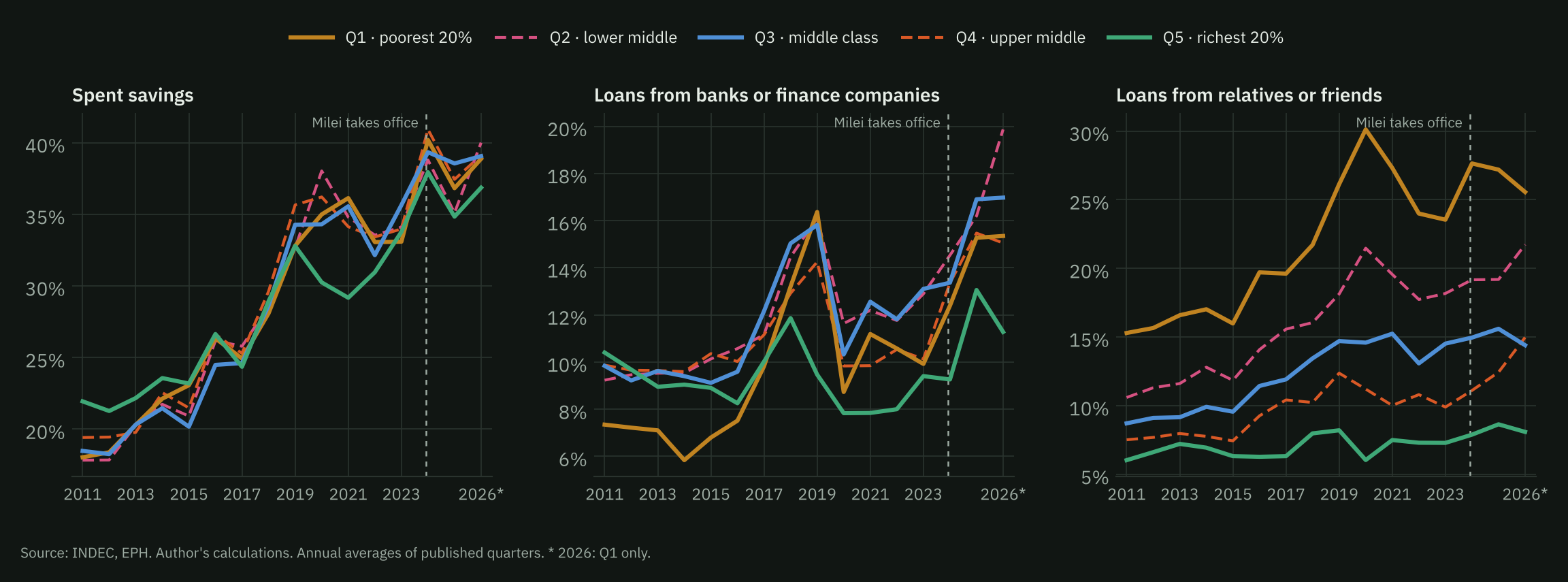
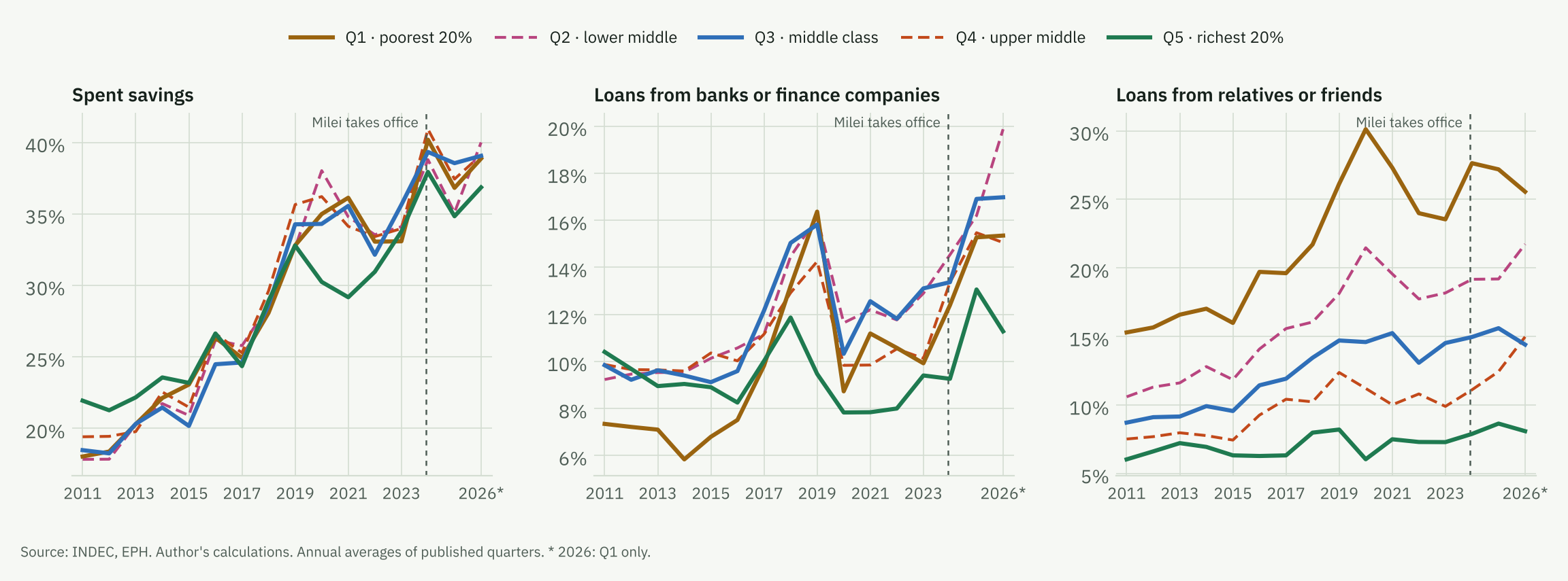
The share of households that lived on their savings went from about a third in 2019 and 2023 to a peak of 38.4% in the first quarter of 2024, the highest since 2003 (the previous peak, 36.7%, was in the second quarter of 2020). In the first quarter of 2026 it was still 36.2%. Loans from banks and finance companies rose later: 14.9% in the fourth quarter of 2025 and 14.8% in the first of 2026, above any quarter up to 2024 (14.0%). The sequence is what one expects if savings are used first and credit afterwards.
| Indicator | Q1 | Q2 | Q3 | Q4 | Q5 | Total |
|---|---|---|---|---|---|---|
| Spent savings | 33.1 → 36.8 | 34.1 → 35.1 | 35.6 → 38.6 | 34.0 → 37.4 | 33.8 → 34.8 | 32.0 → 34.9 |
| Loans from relatives or friends | 23.5 → 27.2 | 18.2 → 19.2 | 14.5 → 15.6 | 9.9 → 12.4 | 7.3 → 8.6 | 13.4 → 15.6 |
| Loans from banks or finance companies | 9.9 → 15.3 | 12.9 → 16.2 | 13.1 → 16.9 | 10.1 → 15.5 | 9.4 → 13.1 | 10.1 → 14.0 |
| Instalment or credit purchases | 37.0 → 39.3 | 45.6 → 44.8 | 49.9 → 53.4 | 57.7 → 56.1 | 66.9 → 63.8 | 49.7 → 49.9 |
| Sold belongings | 14.3 → 15.7 | 9.2 → 10.6 | 8.4 → 10.2 | 5.5 → 7.2 | 5.0 → 5.5 | 8.1 → 9.5 |
By quintile, spending savings is similar across the distribution. Bank credit, by contrast, is highest in the middle class: 16.9% of third-quintile households and 16.2% of second-quintile households in 2025, and 19.9% in the second quintile in the first quarter of 2026. The poorest borrow from relatives or friends (27.2% in 2025) and sell belongings (15.7%). Instalment and credit purchases mix routine card use with borrowing; their trend, not their level, is what matters.
| Indicator | Woman | Man | Low educ. | Mid educ. | Tertiary |
|---|---|---|---|---|---|
| Spent savings | 30.6 → 34.1 | 33.3 → 35.7 | 28.9 → 33.4 | 33.2 → 35.5 | 35.4 → 36.4 |
| Loans from relatives or friends | 13.7 → 16.7 | 13.2 → 14.7 | 15.3 → 18.8 | 13.9 → 15.6 | 9.4 → 10.5 |
| Loans from banks or finance companies | 10.0 → 13.8 | 10.1 → 14.1 | 10.3 → 13.5 | 10.2 → 14.7 | 9.5 → 13.2 |
| Sold belongings | 7.9 → 9.6 | 8.3 → 9.3 | 8.9 → 10.9 | 8.3 → 9.3 | 6.2 → 7.4 |
| Receives a state cash benefit | 17.2 → 17.1 | 14.1 → 13.1 | 23.8 → 23.3 | 14.6 → 14.0 | 3.1 → 3.0 |
| Receives help from relatives or neighbours | 8.1 → 10.2 | 5.8 → 6.6 | 7.8 → 10.6 | 7.7 → 8.3 | 3.8 → 4.3 |
Households whose main earner is a woman rely more on loans from relatives or friends (16.7% against 14.7%) and on help from non-residents. Households whose main earner has little education borrow more from relatives (18.8% against 10.5% with tertiary education) and increased their use of savings the most between 2023 and 2025 (28.9% to 33.4%). Bank credit rose evenly across groups.
Working more
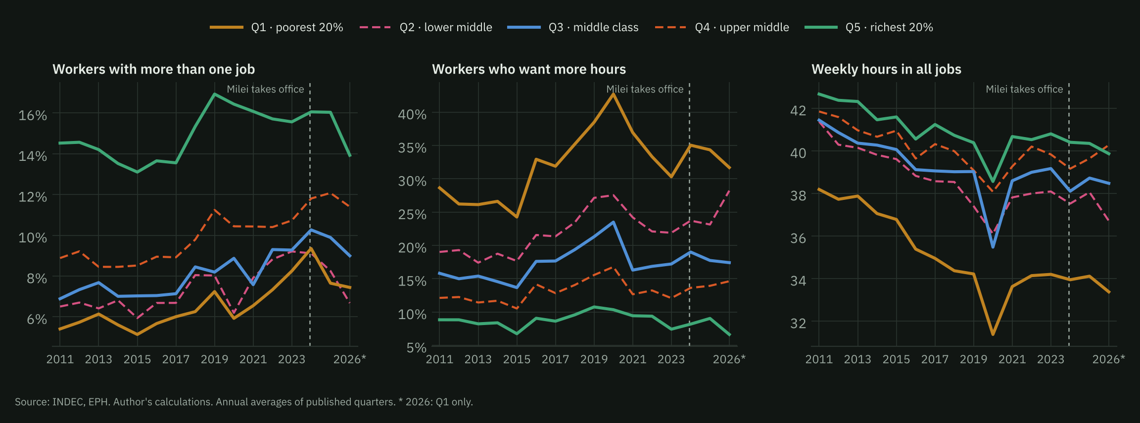
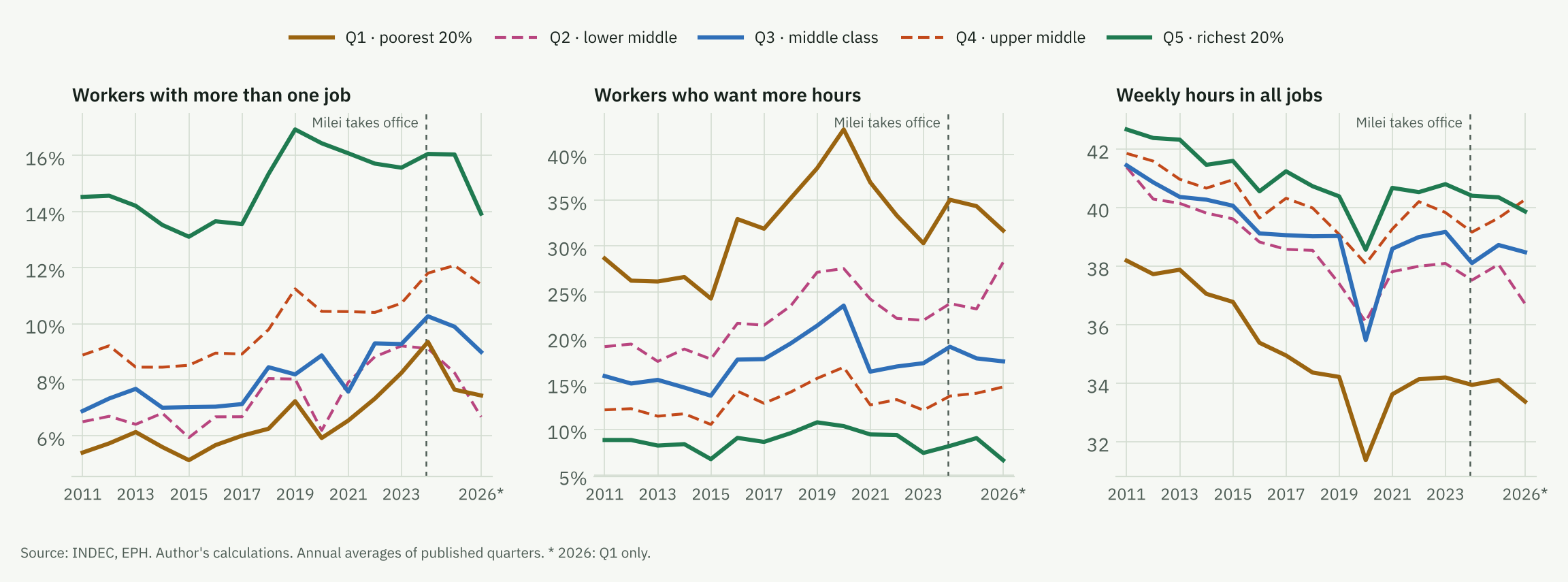
Multiple jobholding averaged 11.5% of workers in 2024 and 11.5% in 2025, the highest annual value since 2003; between 2011 and 2015 it never exceeded 8.8% and in 2017 it was 8.7%. It is higher in the richest quintile (teaching, health, professions) and among women (14.7% against 8.9%), but it grew in every quintile since 2017; between 2023 and 2025 it fell slightly in the first and second, and in the first quarter of 2026 the total stood at 10.4%.
| Indicator | Q1 | Q2 | Q3 | Q4 | Q5 | Total |
|---|---|---|---|---|---|---|
| Has more than one job | 8.2 → 7.7 | 9.2 → 8.3 | 9.3 → 9.9 | 10.7 → 12.1 | 15.6 → 16.0 | 10.8 → 11.5 |
| Weekly hours, all jobs | 34.2 → 34.1 | 38.1 → 38.1 | 39.2 → 38.7 | 39.8 → 39.6 | 40.8 → 40.3 | 38.5 → 38.1 |
| Hours in the second job | 11.9 → 11.6 | 12.9 → 13.3 | 15.4 → 14.3 | 14.6 → 14.8 | 15.3 → 14.4 | 14.2 → 14.2 |
| Works more than 45 hours | 26.9 → 26.8 | 32.5 → 31.8 | 32.2 → 30.2 | 29.9 → 29.0 | 27.6 → 26.8 | 30.0 → 28.9 |
| Wants to work more hours | 30.3 → 34.3 | 21.9 → 23.1 | 17.2 → 17.7 | 12.1 → 13.9 | 7.4 → 9.0 | 17.3 → 19.0 |
| Employee without pension contributions | 68.7 → 67.1 | 46.4 → 45.2 | 34.4 → 31.8 | 22.0 → 23.1 | 14.7 → 15.7 | 36.3 → 36.7 |
Hours did not rise in any quintile: average hours in all jobs were 38.5 in 2023 and 38.1 in 2025. The intensity of the second job did not rise either (14.2 and 14.2 weekly hours among multiple jobholders), and the share working more than 45 hours fell (30.0% to 28.9%). The distribution by hours bands, in the next table, confirms there is no shift towards longer hours in any quintile. What grows is the wish to work more hours: from 17.3% to 19.0% of workers, and from 30.3% to 34.3% in the poorest quintile. Those who take a second job make up for hours lost in the first, or the increase is too small to move the average.
| Group | 1-15 | 16-34 | 35-45 | 46-60 | 61+ |
|---|---|---|---|---|---|
| Q1 · 2017 | 18.2 | 28.4 | 23.7 | 22.3 | 7.4 |
| Q1 · 2023 | 19.2 | 29.6 | 24.4 | 20.9 | 6.1 |
| Q1 · 2025 | 19.0 | 29.8 | 24.4 | 20.1 | 6.6 |
| Q2 · 2017 | 10.3 | 26.5 | 28.7 | 26.8 | 7.7 |
| Q2 · 2023 | 11.0 | 27.6 | 29.3 | 25.1 | 7.1 |
| Q2 · 2025 | 9.7 | 28.2 | 30.7 | 24.7 | 6.6 |
| Q3 · 2017 | 8.5 | 26.1 | 33.0 | 25.2 | 7.2 |
| Q3 · 2023 | 8.3 | 25.5 | 33.9 | 25.3 | 7.0 |
| Q3 · 2025 | 8.0 | 26.6 | 35.1 | 24.2 | 6.2 |
| Q4 · 2017 | 6.0 | 24.6 | 38.1 | 24.2 | 7.1 |
| Q4 · 2023 | 5.5 | 24.8 | 38.9 | 24.8 | 6.0 |
| Q4 · 2025 | 5.8 | 25.0 | 39.7 | 23.4 | 6.2 |
| Q5 · 2017 | 3.9 | 20.0 | 45.8 | 23.8 | 6.3 |
| Q5 · 2023 | 3.4 | 21.0 | 47.2 | 22.2 | 6.0 |
| Q5 · 2025 | 4.1 | 22.8 | 45.3 | 22.1 | 5.8 |
| Indicator | Woman | Man | Low educ. | Mid educ. | Tertiary |
|---|---|---|---|---|---|
| Has more than one job | 14.3 → 14.7 | 8.1 → 8.9 | 8.6 → 8.6 | 8.3 → 8.9 | 18.5 → 20.0 |
| Weekly hours, all jobs | 33.9 → 33.9 | 42.2 → 41.5 | 38.3 → 37.9 | 38.7 → 38.4 | 38.7 → 38.0 |
| Wants to work more hours | 18.8 → 20.7 | 16.1 → 17.7 | 22.6 → 25.0 | 17.1 → 18.5 | 11.1 → 13.1 |
| Employee without pension contributions | 37.9 → 38.4 | 34.9 → 35.4 | 56.4 → 58.0 | 36.1 → 36.5 | 14.5 → 15.8 |
Added worker. The labour force participation of first-quintile spouses rose from 38.3% in 2017 to 47.1% in 2023, following the long-run rise in female participation, and has been flat since (46.8% in 2025); that of children did not move either. To look inside households we use the panels: among people aged 14–64 who are not the main earner and were inactive, we measure the share who start working or looking for work, by how the main earner’s real income changed between the two interviews.
| Main earner’s real income | Active next quarter | Observations | Active one year later | Observations |
|---|---|---|---|---|
| Falls more than 10% | 16.7 | 44,553 | 23.4 | 41,851 |
| Between −10% and +10% | 14.2 | 25,217 | 21.7 | 17,474 |
| Rises more than 10% | 17.4 | 44,047 | 23.5 | 34,776 |
| Main earner loses the job | 13.5 | 15,299 | 15.8 | 14,770 |
Entry into the labour force is somewhat higher when the main earner’s income falls by more than 10% (16.7% by the next quarter) than when it is stable (14.2%), but it is just as high when it rises (17.4%), and lower when the main earner loses the job (13.5%). One year later the pattern is the same (23.4%, 21.7%, 23.5% and 15.8%). The descriptive evidence thus shows no clean added-worker effect: households with volatile incomes move in and out of the labour market more, and the main earner’s job loss may coincide with shocks that hit the whole household (a family business, a depressed local market). Estimating the effect requires comparing similar households before the shock, which is the design of the academic work that follows.
Receiving help
| Indicator | Q1 | Q2 | Q3 | Q4 | Q5 | Total |
|---|---|---|---|---|---|---|
| Receives a state cash benefit | 45.2 → 44.6 | 20.1 → 17.6 | 7.4 → 8.4 | 3.2 → 2.0 | 0.9 → 0.9 | 15.6 → 15.0 |
| Receives food or goods (state, churches, schools) | 19.5 → 19.7 | 8.1 → 8.7 | 4.4 → 4.3 | 1.8 → 1.3 | 0.6 → 0.2 | 6.6 → 7.0 |
| Receives help from relatives or neighbours | 11.1 → 12.7 | 7.7 → 9.3 | 7.3 → 7.2 | 5.1 → 5.6 | 1.9 → 2.4 | 6.9 → 8.3 |
| A member receives a state transfer | 45.1 → 44.6 | 20.1 → 17.5 | 7.4 → 8.3 | 3.2 → 2.0 | 0.9 → 0.8 | 15.3 → 14.5 |
| Real transfer per recipient household (thousand $ of Q1 2026) | 235 → 292 | 196 → 228 | – | – | – | 214 → 268 |
| Transfers / household income | 14.5 → 16.1 | 2.7 → 2.5 | 0.7 → 0.8 | 0.2 → 0.1 | 0.0 → 0.1 | 3.6 → 3.9 |
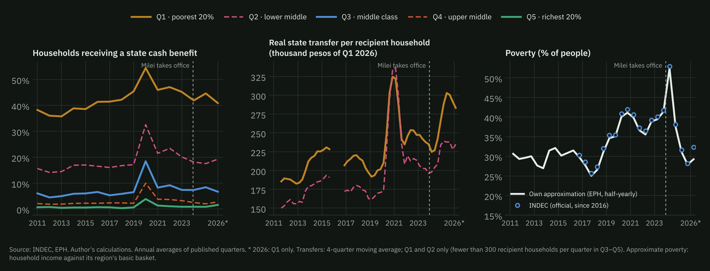
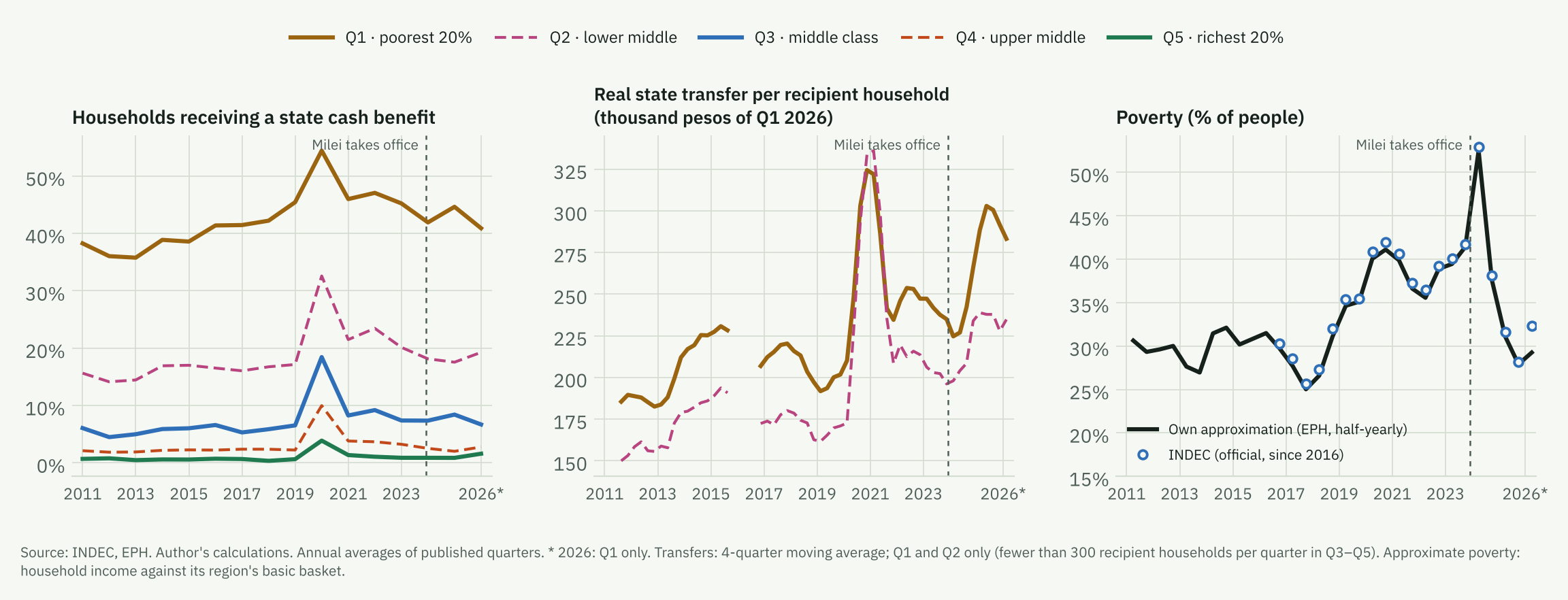
In the first quintile, the share of households living partly on a state cash benefit is high and stable (45.2% in 2023 and 44.6% in 2025); AUH alone reaches 42.0%. What changed is the amount. The real transfer per recipient household was 24.1% higher in 2025 than in 2023 in the first quintile, and went from 14.5% to 16.1% of total household income. The quarterly series shows a fall in late 2023 and early 2024, as inflation accelerated, a strong rise during 2024 and a gradual decline in 2025: in the first quarter of 2026 the real amount was still 18.1% above the third quarter of 2023. The 2020 peak corresponds to the Emergency Family Income (IFE; smoothed by the moving average in the figure).
Food and goods from the state, churches or schools became common during the pandemic and did not return to the earlier level (7.3% of first-quintile households in 2019, 19.7% in 2025). Help from relatives or neighbours rose from 6.9% to 8.3% of households.
| Half-year | INDEC official | Own approximation | Without state transfers | Difference (points) |
|---|---|---|---|---|
| 2017 H1 | 28.6 | 27.7 | 29.5 | 1.8 |
| 2017 H2 | 25.7 | 25.0 | 26.4 | 1.4 |
| 2018 H1 | 27.3 | 26.6 | 28.2 | 1.6 |
| 2018 H2 | 32.0 | 31.1 | 32.3 | 1.3 |
| 2019 H1 | 35.4 | 34.6 | 36.1 | 1.5 |
| 2019 H2 | 35.5 | 35.1 | 36.2 | 1.1 |
| 2020 H1 | 40.9 | 40.1 | 42.9 | 2.8 |
| 2020 H2 | 42.0 | 41.1 | 45.6 | 4.5 |
| 2021 H1 | 40.6 | 39.9 | 41.4 | 1.5 |
| 2021 H2 | 37.3 | 36.6 | 38.5 | 1.9 |
| 2022 H1 | 36.5 | 35.6 | 38.0 | 2.5 |
| 2022 H2 | 39.2 | 38.9 | 40.7 | 1.8 |
| 2023 H1 | 40.1 | 39.5 | 41.1 | 1.7 |
| 2023 H2 | 41.7 | 41.4 | 42.8 | 1.3 |
| 2024 H1 | 52.9 | 52.5 | 53.1 | 0.6 |
| 2024 H2 | 38.1 | 37.6 | 39.4 | 1.9 |
| 2025 H1 | 31.6 | 31.1 | 33.2 | 2.1 |
| 2025 H2 | 28.2 | 27.9 | 30.4 | 2.5 |
| 2026 H1 | 32.3 | 29.3 | 32.4 | 3.1 |
According to INDEC, poverty among people went from 41.7% in the second half of 2023 to 52.9% in the first half of 2024, fell to 28.2% in the second half of 2025 and rose to 32.3% in the first half of 2026. The own approximation follows that path. The mechanical counterfactual, which subtracts state cash transfers from household income with no behavioural response, implies that without them poverty would have been 1.5 points higher in 2023, 2.3 points in 2025 and 3.1 points in the first quarter of 2026; since 2024, almost all of the difference is due to AUH. Transfers therefore underpin the measured poverty level: part of the improvement of the poorest households lies in them rather than in the labour market.
Consuming less or worse
The EPH does not measure consumption, but it shows two important items: schooling, following the same people for a year, and health coverage.
| Indicator | 2017 | 2018 | 2019 | 2021 | 2022 | 2023 | 2024 | 2025 |
|---|---|---|---|---|---|---|---|---|
| Private to public within a year · Total | 22.4 | 21.2 | 17.5 | 23.7 | 18.7 | 17.8 | 17.7 | 20.4 |
| Private to public within a year · Woman | 23.2 | 22.1 | 17.3 | 22.5 | 19.1 | 18.8 | 20.0 | 21.3 |
| Private to public within a year · Man | 21.5 | 20.2 | 17.6 | 24.7 | 18.3 | 16.7 | 15.4 | 19.5 |
| Pupils in private school · Total | 29.2 | 29.3 | 31.5 | 27.2 | 30.2 | 28.4 | 27.8 | 27.2 |
| Pupils in private school · Woman | 30.9 | 30.0 | 34.2 | 27.0 | 30.3 | 29.7 | 27.0 | 28.0 |
| Pupils in private school · Man | 27.5 | 28.6 | 28.9 | 27.4 | 30.0 | 27.2 | 28.6 | 26.5 |
| Leave school, ages 13–16 · Total | 5.2 | 5.1 | 3.1 | 3.1 | 2.6 | 2.7 | 3.3 | 3.2 |
| Leave school, ages 13–16 · Woman | 4.0 | 4.4 | 2.6 | 2.8 | 2.0 | 2.1 | 2.4 | 3.5 |
| Leave school, ages 13–16 · Man | 6.4 | 5.8 | 3.7 | 3.3 | 3.1 | 3.3 | 4.1 | 2.9 |
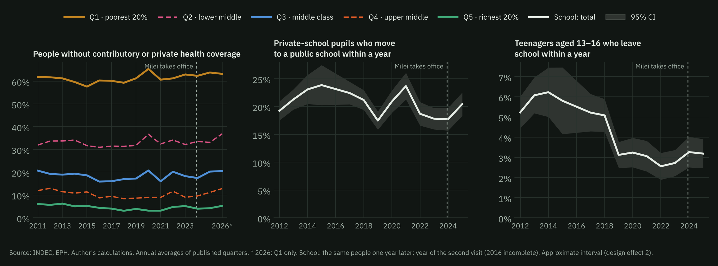
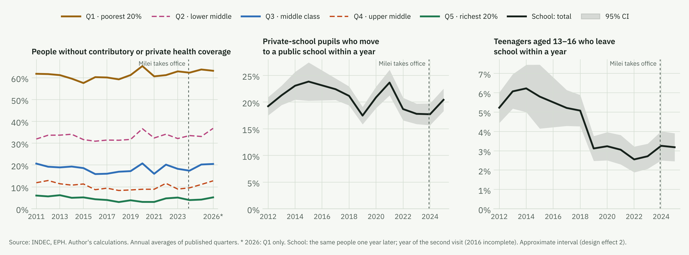
School. The share of private-school pupils who moved to a public school within a year was 20.4% in 2025 (2,831 private-school pupils at the first visit), against an average of 18.1% in 2022–2024. The difference is at the edge of statistical significance (z = 1.9; margin of error of the 2025 figure: ±2.1 points). It is not a historical high: the peak was 23.7% in 2021. There is no difference by gender (z = 0.9). One-year dropout among teenagers aged 13–16 was 3.2% in 2025 (4,526 teenagers), against 2.8% in 2022–2024 (z = 0.8): there is no increase. The previous version of this report highlighted a rise in the first quintile; with 1,638 teenagers in that quintile in 2025 the error exceeds one point and year-to-year jumps cannot be told apart from noise, so it is no longer reported. The break in the series between 2018 and 2019 has no clear explanation in the data and is read with caution. 2026 (only pairs whose second visit is the first quarter) is not used: the first quarter coincides with the change of school year.
| Indicator | Q1 | Q2 | Q3 | Q4 | Q5 | Total |
|---|---|---|---|---|---|---|
| No contributory or private health coverage | 63.2 → 63.2 | 29.0 → 36.8 | 19.5 → 20.5 | 9.4 → 12.8 | 4.3 → 5.2 | 32.0 → 34.1 |
| Contributory health insurance | 32.1 → 31.9 | 65.5 → 60.4 | 75.5 → 74.1 | 84.8 → 81.3 | 83.4 → 78.8 | 61.5 → 59.6 |
| Private or mutual health plan | 2.8 → 1.4 | 5.1 → 1.9 | 5.1 → 6.3 | 8.2 → 7.5 | 17.5 → 19.8 | 7.1 → 6.3 |
Health. With annual averages, the share of people without contributory or private health coverage went from 31.7% in 2023 to 32.7% in 2025, and was 34.1% in the first quarter of 2026 (32.0% in the same quarter of 2023). The annual rise is concentrated in the third quintile (18.3% to 20.2%) and the fourth (9.0% to 11.1%); in the second, the first-quarter comparison shows a larger jump (29.0% to 36.8%) than the annual average (32.1% to 33.1%), and private plans also fell there (4.9% to 2.9%). This is consistent with less registered employment and with higher private-plan fees after their deregulation in December 2023, but the data cannot separate the two. In the panel, the “private plan” category is often reclassified as “contributory insurance” because of response error; the cross-section is used instead.
Other consumption. The EPH does not ask about food, brands, services or leisure. Switching to cheaper brands, wholesalers or smaller packages appears in consumer-goods market data and in the crisis literature (McKenzie and Schargrodsky, 2011; Jaimovich, Rebelo and Wong, 2019); this report has no figures of its own on that. Private sources point the same way: mass consumption fell 2.9% in the first half of 2026 and its index is 17.1% below January 2023 (Scentia); in the fourth quarter of 2025 purchase frequency fell 8.2% and volume 4.7%, with value brands as a refuge (Worldpanel by Numerator); beef consumption is 47.3 kg per person per year, against 69.4 in 2008 (CICCRA). Online mass-consumption sales grow fast (41.0% year on year in June 2026, Scentia), but according to the Argentine E-commerce Chamber they reach about 10% of sales in most firms, so they do not offset the fall measured in physical channels.
Relative prices
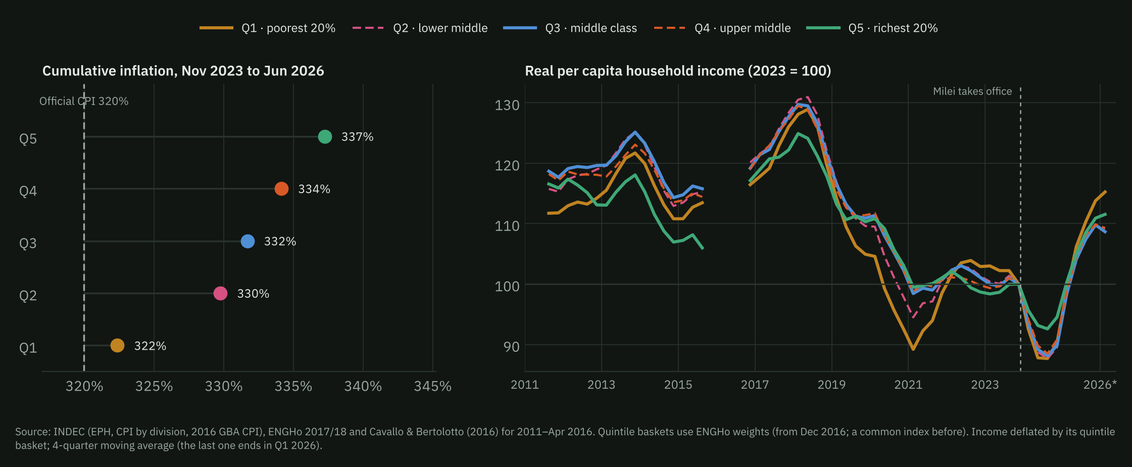
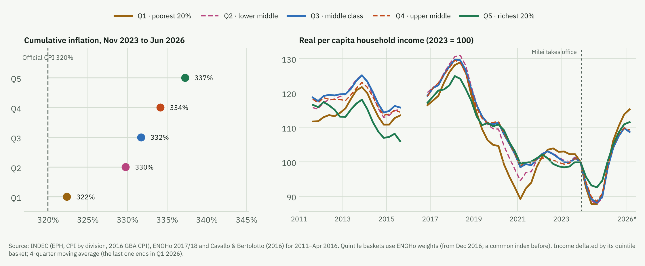
The official CPI uses 2004/05 expenditure weights. To measure how much the cost of each group’s basket changed, a Laspeyres index by quintile is built with the ENGHo 2017/18 shares and the CPI by division.
| Division | Inflation Nov-23 to 06-26 | Weight Q1 | Weight Q3 | Weight Q5 |
|---|---|---|---|---|
| Food and beverages | 293 | 34.5 | 25.4 | 15.7 |
| Housing and utilities | 602 | 14.2 | 14.6 | 14.6 |
| Transport | 383 | 10.4 | 13.2 | 15.6 |
| Health | 334 | 4.2 | 6.1 | 8.0 |
| Education | 443 | 1.6 | 3.1 | 3.8 |
| Communications | 427 | 5.0 | 5.7 | 4.6 |
| Restaurants and hotels | 355 | 4.4 | 5.9 | 8.2 |
Between November 2023 and June 2026 the first-quintile basket rose 322% and the fifth-quintile basket 337% (official CPI: 320%). The difference comes from composition: food (293%) weighs 34.5% in first-quintile spending and 15.7% in fifth-quintile spending, and the largest increases were in housing and utilities (602%), education (443%) and communications (427%). Housing weighs about the same in every quintile: the gap comes mostly from the smaller weight of food at the top. Since wages and pensions are adjusted, at best, by the general CPI, a rise equal to official inflation does not compensate households whose basket rises more. External cross-check: using the ENGHo 2017/18 basket, CP Consultora estimated inflation 12.2 points above the official figure between November 2023 and June 2025 (Letra P); this report’s index, for all households, gives a gap of the same order.
Real income by quintile
| Group | 2017 | 2019 | 2024 | 2025 | Q1 2026 (vs Q1 2023) | 2025, official CPI |
|---|---|---|---|---|---|---|
| Q1 | 126.0 | 104.9 | 90.3 | 113.8 | 109.5 | 114.4 |
| Q2 | 128.3 | 109.6 | 89.5 | 109.7 | 104.5 | 111.4 |
| Q3 | 127.7 | 110.9 | 89.9 | 109.8 | 103.1 | 111.9 |
| Q4 | 127.2 | 111.4 | 90.8 | 109.9 | 106.3 | 112.3 |
| Q5 | 122.2 | 110.3 | 94.5 | 110.9 | 107.4 | 114.1 |
| Total | 124.9 | 110.3 | 92.3 | 110.5 | 106.3 | 113.1 |
With its own quintile basket, real per capita household income in 2025 was 13.8% higher than in 2023 in the first quintile, 10.9% in the fifth and between 9.7% and 9.9% in the three middle quintiles. In the first quarter of 2026, against the same quarter of 2023: first quintile 9.5%, second 4.5%, third 3.1%, fourth 6.3% and fifth 7.4%. Compared with 2017 every quintile is still below, the middle ones the most (14.6% the second, 14.0% the third and 13.6% the fourth, against 9.7% the first and 9.2% the fifth). The profile is U-shaped: the extremes recovered more than the middle. In the first quintile, the rise in the real value of transfers accounts for about 3.5 points of the 2023–2025 improvement (2023 transfer share of income times the real change in the amount per recipient household, with stable coverage). With the official CPI, every group’s recovery looks somewhat larger.
Income capture. The rise in real income measured by the EPH since 2024 exceeds that in administrative records. In the fourth quarter of 2025, the wage of registered employees in the EPH rose 42.7% year on year, against 32.0% in SIPA, 37.0% in RIPTE, 30.0% in INDEC’s wage index and inflation of 31.5% (Equilibra, as reported by Infobae). CEDLAS estimates that, correcting for under-reporting by source, the timing mismatch between incomes and baskets, and the Engel coefficient from ENGHo 2017/18, poverty would have fallen by about 2.0 points between the second half of 2023 and the first half of 2025, not ten. The most cited explanation is that under very high inflation respondents under-report their income more, and that disinflation reversed this bias. For this report, the consequence is that real income levels for 2024–2026 are probably overstated relative to 2023 in every quintile. If the bias is similar across quintiles, as Equilibra suggests (“it is everyone”), the ranking between groups — the result that matters here — does not change; there is no published evidence by quintile to check this.
Informality. The government attributes the real wage recovery to informal workers. In the EPH, real income from the main job (P21, deflated by the official CPI) rose between 2023 and 2025 by 24.3% among unregistered employees, 29.4% among the self-employed and 12.7% among registered employees; against 2017, all three groups are still below (6.8%, 7.9% and 12.9%). The levels match those published by INDEC for the first quarter of 2026 (mean income of $727,000 and $1,372,000 for unregistered and registered employees, against INDEC’s $731,000 and $1,375,000; unregistered share of employees: 37.9%, against 37.9%). INDEC’s unregistered wage index, which shows a real rise of 84.0% since November 2023 according to Tiempo Argentino, faces three criticisms: it is built from the same EPH and reflects incomes about 6 months earlier, so it compares periods with different inflation (Pastrana, C-P); it inherits the survey’s improved income capture, which for non-employees shows 70.0% year on year at the end of 2025 (Equilibra); and it is inconsistent with other employment and consumption indicators (Maito, CETyD-UNSAM; Campos, CTA Autónoma). On the administrative side, registered wage employment fell by 205,000 jobs between November 2023 and July 2025 (IIEP-EDIL, UBA). The robust part is that informal income recovered more than formal income relative to 2023, from a very low floor, is still about half of it (48% of registered pay in 2025) and has not returned to its 2017 level.
Why 2017. 2023 is a low base (triple-digit inflation and income under-reporting). 2017 is the last year with inflation of the current order before the 2018 crisis, and it is the purchasing-power reference families have. Under high inflation, prices lose informational content and real comparisons become hard (Heymann and Leijonhufvud, 1995); disinflation makes them possible again. This is a hypothesis consistent with the ‘nominal memory’ Equilibra uses to explain 2023 under-reporting, not a result of this report.
Limits of the quintile index. ENGHo quintiles are of households and EPH quintiles of people: the match is approximate. The index uses a fixed basket, with no substitution, so it is an upper bound on the difference between groups. The published ENGHo does not cross quintile with region, and region matters because utility tariffs rose more in the Buenos Aires metropolitan area.
Synthesis: the four channels
The channels do not all push in the same direction, and that is why the pressure concentrates on the middle class.
- Receiving help is progressive: state transfers are 16.1% of first-quintile income and almost nothing above the second; their real value rose (24.1% per first-quintile recipient household, 2025 against 2023).
- Relative prices go the other way: the basket became more expensive the higher the income (322% in the first quintile, 332% in the third and 337% in the fifth, against 320% for the official CPI).
- Real income, deflated by each group’s own basket, combines both and is U-shaped: the extremes recovered more than the middle. It is not that the rich did best: the first quintile rose most, the fifth followed, and the second and third rose least.
- Borrowing and dissaving: dissaving was even; bank credit peaks in the second and third quintiles; at the bottom, help from relatives and selling belongings.
- Working more: more jobs, not more hours; multiple jobholding kept rising after 2023 only in the third and fourth quintiles; unmet demand for hours grows mostly at the bottom. No clear added-worker effect.
- Consuming worse: the loss of health coverage concentrates in the third and fourth quintiles; schooling gives a weak signal.
The conclusion that the middle class bears the strongest pressure does not come from a single channel but from their combination: it does not receive the help that protects the bottom, it faces basket inflation almost as high as the top without the top’s cushion, and so its real income recovered least; and the strategies that depend on the household itself — bank credit, loss of health coverage, a second job — concentrate there. None of this shows up in the poverty rate, which measures the distance to a line, not the cost of staying above it.
Next steps
- Added worker and dropout with Latin American panels since 2003. Extend the design of Ciaschi and Neidhöfer (2024), which ends in 2015 and uses only Argentina and male heads: every country with a panel, a main earner of either gender, their own labour supply and that of the other members, and household strategies as outcomes.
- Continuous erosion of the real wage. Continuous treatment: the change in the real wage of the main earner’s industry (registered employees’ pay by industry and province, deflated by the quintile index) between panel visits; difference-in-differences with a continuous treatment (Callaway, Goodman-Bacon and Sant’Anna, 2024) and threshold estimation (Hansen, 2000).
- Transfers and poverty. Reproduce the official half-yearly measurement and separate the contributions of AUH, other programmes and pensions; contrast EPH incomes with administrative records by quintile.
- Consumption. Match the EPH with the ENGHo as a compositional counterfactual.
References
- Cavallo, A. and Bertolotto, M. (2016). Filling the gap in Argentina’s inflation data. MIT Sloan / PriceStats. Series at inflacionverdadera.com/Argentina_inflation.csv.
- Callaway, B., Goodman-Bacon, A. and Sant’Anna, P. H. C. (2024). Difference-in-differences with a continuous treatment. NBER Working Paper 32117.
- Chequeado (2025). AUH: cuál es el aumento en diciembre de 2025 y cómo evolucionó el monto de la asignación. El Explicador.
- Ciaschi, M. and Neidhöfer, G. (2024). Job loss and household labor supply adjustments in developing countries: Evidence from Argentina. The World Bank Economic Review, 38(3), 558–579.
- Dessing, M. (2002). Labor supply, the family and poverty: the S-shaped labor supply curve. Journal of Economic Behavior & Organization, 49(4), 433–458.
- Heymann, D. and Leijonhufvud, A. (1995). High Inflation: The Arne Ryde Memorial Lectures. Oxford: Clarendon Press.
- Hansen, B. E. (2000). Sample splitting and threshold estimation. Econometrica, 68(3), 575–603.
- Infobae (2026a). El cambio del Indec en la medición de ingresos distorsionó el dato de baja de la pobreza, según un estudio privado (7 April).
- Infobae (2026b). Las cifras de la pobreza en la Argentina: por qué la baja de los indicadores desató un intenso debate entre economistas (14 April).
- INDEC (2016). La medición de la pobreza y la indigencia en la Argentina. Metodología INDEC 22.
- INDEC (2026). Incidencia de la pobreza y la indigencia en 31 aglomerados urbanos. Primer semestre de 2026.
- Jaimovich, N., Rebelo, S. and Wong, A. (2019). Trading down and the business cycle. Journal of Monetary Economics, 102, 96–121.
- Jaravel, X. (2021). Inflation inequality: Measurement, causes, and policy implications. Annual Review of Economics, 13, 599–629.
- Kaplan, G. and Schulhofer-Wohl, S. (2017). Inflation at the household level. Journal of Monetary Economics, 91, 19–38.
- Letra P (2025). Indec: el nuevo IPC está listo, da más alto y el FMI permitió patearlo después de las elecciones.
- Lundberg, S. (1985). The added worker effect. Journal of Labor Economics, 3(1), 11–37.
- McKenzie, D. and Schargrodsky, E. (2011). Buying less but shopping more: The use of nonmarket labor during a crisis. Economía, 11(2), 1–43.
- IIEP-EDIL (2025). Panorama del empleo asalariado formal y de las remuneraciones. Instituto Interdisciplinario de Economía Política, UBA, October.
- Paz, J. A. (2009). El efecto del trabajador adicional. Evidencia para Argentina (2003–2007). Cuadernos de Economía, 46(134), 225–241.
- Press cited for figures from other sources: BAE Negocios (23/7/2026, Scentia), Infobae (30/3/2026, Worldpanel by Numerator), El Ancasti (19/3/2026, CICCRA), El Cronista (29/4/2026, CACE), Tiempo Argentino (6/9/2026, unregistered wage index).
- Stephens, M. (2002). Worker displacement and the added worker effect. Journal of Labor Economics, 20(3), 504–537.
Data: INDEC (Permanent Household Survey, CPI by division, ENGHo 2017/18, total basic basket and poverty reports). INDEC’s original microdata; household file harmonised by the Encuestas LATAM project. Prices 2011–2016: Cavallo and Bertolotto (2016) and INDEC’s Greater Buenos Aires CPI. Every figure comes from reproducible code; code and intermediate data are available on request.